Multi-Orient Extraction (multi)

The multi-orient extraction was first developed by Ryan, Casertano, & Pirzkal (2018) and referred to as LINEAR. This method was founded to address the contamination (or confusion) from overlapping spectral traces, where the detector records a weighted sum of the the spectra (see Fig. 5.4 below). Therefore, this represents a fundamental degeneracy, which can only be broken with additional data. The single-orient extraction formalism uses the broadband data to inform the contamination model, whereas the LINEAR uses data at multiple orients provide a self-consistent, spectroscopic model for the entire scene.

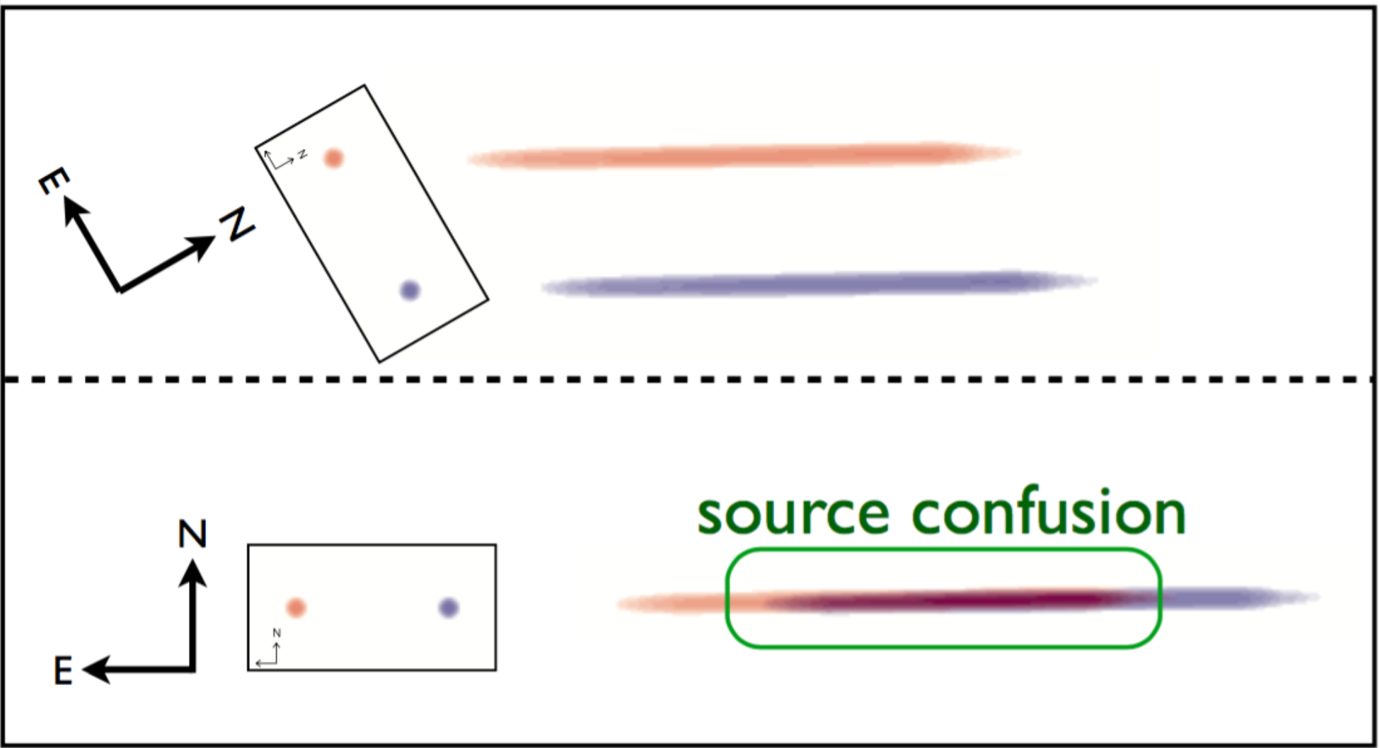
Fig. 5.4 An illustration of spectral contamination or confusion (taken from Ryan, Casertano, & Pirzkal 2018). Along the left side of each panel, they show a red and blue point source whose celestial positions are fixed (as shown the coordinate vane). This shows that under certain orients (lower panel), the spectra will overlap leading to the spectral degeneracy. However, if the telescope is reoriented, then the spectral traces separate, which provides the leverage to break this degeneracy.

Although the formative effort was to break the degeneracy from contamination/confusion, additional advantages were identified. Namely, the spectral resolution of a WFSS mode, is set by properties of the grating and the size of the source. In analogy to the relationship between slit width and spectral resolution for long-slit spectroscopy, the size of the source projected along the dispersion axis set the resolution — where the larger the source, the lower the resolution. Therefore, simply averaging spectra extracted at separate orients (such as described in single-orient extraction) will result in biases, when the resolutions are different (which most often occurs for extended sources). Hence, one can either smooth all the data to a common resolution before averaging (which loses spectral resolution) or analyze the high-resolution data by itself (which loses signal-to-noise). But Ryan, Casertano, & Pirzkal (2018) find that the LINEAR method recovers the highest spectral resolution present in the data, at the cost of an increased computational resources and collecting data at multiple orients.

Mathematical Formulation

The LINEAR framework acknowledges that the flux in a WFSS image pixel is the sum of all sources and wavelengths, weighted by factors related to the sources (e.g. the cross-dispersion profiles) and the detector (e.g. sensitivity curve, flat-field, or pixel-area map):

\[S_{x,y,i} = \sum_{l}\sum_{k=1}^{N_\mathrm{obj}} W_{x,y,i,l,k}\, f_{l,k}\]

where \(i\) refers to the \(i^{\rm th}\) WFSS image in the collection. The known and unknown indices are grouped together with np.ravel_multi_index() as:

\[\begin{split}\begin{aligned} \vartheta &=& x + n_x\,y+ n_x\,n_y\,i\\ \varphi &=& l + n_l\,k \end{aligned}\end{split}\]

respectively. Now the above double sum is recast as a simple matrix equation:

\[S_{\vartheta} = \sum_\varphi W_{\vartheta,\varphi}\, f_{\varphi}.\]

But since this is an overconstrained problem, then the vector of unknowns \(f_{\varphi}\) must be solved with optimization techniques:

\[\chi^2\left(f_\varphi\right) = \sum_{\vartheta} \left(\frac{S_{\vartheta} - \sum_{\varphi} W_{\vartheta,\varphi}\,f_{\varphi}}{U_{\vartheta}}\right)^2\]

which is simplified by subsuming the WFSS uncertainties into the data and linear operator as:

\[\begin{split}\begin{aligned} S_{\vartheta} &\rightarrow& \frac{I_{\vartheta}}{U_{\vartheta}}\\ W_{\vartheta,\varphi} &\rightarrow& \frac{W_{\vartheta,\varphi}}{U_{\vartheta}} \end{aligned}\end{split}\]

so that now \(\chi^2(f_{\varphi}) = ||I - W\,f_{\varphi}||^2\). Although this can be directly solved, the poor condition number of \(W\) can amplify the input noise into the output result, which can be ameliorated by including a regularization term. Additionally, for most WFSS observations, the linear operator \(W\) will be extremely sparse, which permits specialized techniques to iteratively compute the unknown vector \(f_{\varphi}\) without computing the pseudo-inverse of \(W\). However, Ryan, Casertano, & Pirzkal (2018) re-frame the regularization term so that the regularization parameter becomes dimensionless.

\[\psi^2(f_{\varphi};\ell) = \chi^2(f_{\varphi}) + \ell\,\xi^2(f_{\varphi})\]

where \(\ell\) is the regularization parameter and the regularization term is

\[\xi^2\left(f_\varphi\right) = ||W||_F^2\,\sum_\varphi\left(f_{\varphi}-f_{\varphi}^{(0)}\right)^2\]

with \(||W||_F\) is the Frobenius norm and \(f_{\varphi}^{(0)}\) is the damping target, which is initialized from the broadband data. Now the goal is to find the vector \(f_\varphi\) that minimizes \(\psi^2\) for a choice of \(\ell\).

The Role of the Damping Target

The damping target predominately controls how the spectra behave near the edges of the WFSS sensitivity curve. The default behavior is to damp to the broadband photometry, which will lead to spectra that tend to the photometry. In Fig. 5.5, we show an example of this using a source with a flat spectrum: \(f_{\lambda}\sim6.1\times10^{-17}~\mathrm{erg}/\mathrm{s}/\mathrm{cm}^2/\mathrm{Å}\) as a dotted black line.

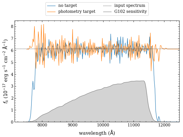
Fig. 5.5 Example of the role of the damping target. The true spectrum is shown as a dotted black line (taken to be a constant of \(\sim6.1\times10^{-17} \mathrm{erg}/\mathrm{s}/\mathrm{cm}^2/\mathrm{Å}\) or \(m_{\mathrm{AB}}=18\) mag), and the extractions with no damping target (blue) and a constant equal to the broadband flux (orange). The light gray region shows the throughput curve of the G102 grism on WFC3/IR. The solver algorithm will attempt to extrapolate the spectrum equal to the damping target, therefore the “no-damping target” case (blue) will tend to zero. On the other hand, the damping target set to the broadband photometry (orange) will tend to that value, which will produce spectra that better match the photometry.

Note

The damping target can be changed by slitlessutils.core.modules.extract.multi.Matrix.set_damping_target(), and future versions will improve this functionality.

Notes on the Uncertainties

Based on the above mathematical formulation, the linear-reconstruction methods will produce uncertainties as the diagonals of the matrix:

\[u_{\varphi}^2 = \mathrm{diag}\left({\left(W^\mathrm{T}W+\ell^2||W_F||^2\right)^{-1}}\right)\]

However, the propagation of uncertainties that accounts for only the detector/astrophysical effects should come from the diagonal elements of \(\sqrt{\left(W^\mathrm{T}W\right)^{-1}}\) (ie. \(\ell=0\)). Therefore for \(\ell\neq0\), the uncertainties will be underestimated. In any case, although the matrix \(W\) is constructed to be sparse, the product with its transpose \(W^\mathrm{T}\) is not guaranteed to be sparse. Therefore these estimates for \(u_{\varphi}\) are compute iteratively, without explicitly computing \(W^\mathrm{T}W\).

Warning

The uncertainties produced in the linear-reconstruction method are generally underestimated. Future releases will implement a Markov-Chain Monte Carlo (MCMC) method to give more realistic uncertainties.

Sparse Linear-Operator Construction

The sparse linear-operator is constructed internally using scipy.sparse.csr_matrix(), which is very convenient for removing rows that have all zeros. Such rows refer to observed pixels that have no spectral information (ie. contain only sky background). Internally a CSR matrix is created for each source for each WFSS image, which are stacked to create a complete CSR matrix (see Griggio et al. 2026 for more details). After creating a full matrix, it is converted to a scipy.sparse.csc_matrix() to identify columns that are all zeros. An all-zero column represents a spectral element that has no observed constraints, which will be returned as np.nan.

Sparse Least-Squares Solution

There have been several algorithms devised to find the vector \(f_{\varphi}\) that minimizes the cost function for \(\psi^2\), and many have been implemented into the scipy sparse solvers. However, slitlessutils is only organized to work with the two most common methods:

• LSQR: first presented by Paige & Saunders (1982) is the standard tool for these types of linear systems. See also the scipy implementation of LSQR

• LSMR: later developed by Fong & Saunders (2011), and improves upon LSQR by generally converging faster. See also the scipy implementation of LSMR.

Warning

Based on experimentation with the LINEAR work, the LSQR solver generally yields better results at increased CPU costs. Therefore, it is set as the default sparse least-squares solver.

Regularization Optimization

As discussed above, the regularized least-squares introduces a tunable parameter that trades between modeling the data (ie. the \(\chi^2\)-term) and damping the high frequency noise present in inverse problems (ie. the \(\xi^2\)-term). However, there have been heuristic approaches at “optimizing” the regularization parameter \(\ell\), and the most common method is to consider a plot of \(\log\xi^2\) versus \(\log\chi^2\), which often called the “L-curve” as it shows a characteristic sharp resembling a capital-L (see Fig. 5.6). It is accepted that the vertex of the L is represents a good compromise, and so there are several techniques to honing in on this critical point. In broad terms, these methods all rely on some aspect of the finding the point of maximum curvature [1] (lower panel of Fig. 5.6) along the parametric curve (upper panel of Fig. 5.6). Slitlessutils offers three options for identifying this critical point:

1. Single-value: Accept a single value of the regularization parameter, and return the vector \(f_{\varphi}\).

2. Brute-force search: Define a linear grid of \(\ell\), find the \(f_{\varphi}\) that minimizes \(\psi^2\), and compute the curvature [1] at all points. Then return the values of \(f_{\varphi}\) and \(\ell\) that maximize the curvature.

3. Golden-ratio search: Cultrerra & Callegaro present a method based on subdividing the search space by various factors of the golden ratio to minimize unnecessary calls to the sparse least-squares solver and use fewer steps than a brute-force approach.

Note

The Golden search method converges the fastest and produces the best results, and so it is set as the default regularization optimizer.

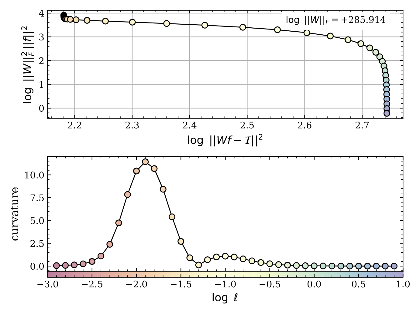
Fig. 5.6 The top panel shows the standard L-curve with the scaling factor of the Frobenius norm to ensure that the regularization parameter \(\ell\) is dimensionless, which is encoded in the color of the plot symbols (see colorbar at the very bottom). The lower panel shows the curvature [1] as a function of the log of the (dimensionless) regularization parameter. The clear peak at \(\log\ell\sim-1.9\) represents the sharp vertex in the L-curve at \((\log\chi^2,\log\xi^2)\sim(2.1,3.6)\). This point is adopted as it represents a roughly “equal” compromise between modeling the data (ie. the \(\chi^2\)-term) and damping high-frequency structure (ie. the \(\xi^2\)-term). This plot was made using the grid-based search with \(\Delta\log\ell=0.1\).

Important

It may be that the resultant spectra show high-frequency oscillations, which is usually a sign the damping was not sufficiently optimized. Users should change the range and tolerance of the damping optimization.

Grouping

As framed above, the multi-orient extraction simultaneously solves for the spectra for entire collection of sources, which depending on the number of sources and/or number of wavelength elements, can result in quite sizeable linear operators. Obviously this would require significant computing resources, something that may not be available. Therefore, slitlessutils has a grouping submodule that will group any spectral traces that overlap in all combinations of the WFSS data together, and these groups can be considered “atomic” problems that can be sequentially solved with significantly less computing resources. This can be thought of as block diagonalizing this sparse operator into chunks that are also sparse systems. See the Grouping Module for more details.

Example

import slitlessutils as su

# load the grism images
data = su.wfss.data.WFSSCollection.from_glob(f'i*flt.fits.gz')

# load the sources into SU
sources = su.sources.SourceCollection('seg.fits', 'sci.fits', local_back=False)

# test grouping
grp = su.modules.Group(ncpu=1, orders=('+1',))
groups = grp(data, sources)

# run the multi-orient extraction using grid-based optimization
# of the L-curve
ext = su.modules.Multi('+1', (-6., -1., 0.1), root='test', algorithm='grid')

# run the extraction with the grouping on
grp_result = ext(data, sources, groups=groups)

# run the extraction with the grouping off
result = ext(data, sources)

Footnotes

[1] (1,2,3)

The curvature is adopted as the Menger curvature.