6. Calibrations for WFSS
The calibration files for slitlessutils are staged on a centralized box repository, which can be accessed using the Config() object. For more information, please see the configuration documentation.
6.1. Spectral Specification
For most operations with WFSS data, we must specify the Spectral Trace and the Spectral Dispersion, which are each given as parametric curves (as described in Pirzkal and Ryan 2017). In brief, here a parameter: \(0 \leq t \leq 1\) describes the \((x(t), y(t),\lambda(t))\). However, these functions can vary within the field-of-view, which is parametrized by the undispersed position \((x_0,y_0)\).
6.1.1. Spectral Trace
The spectral trace describes the position of the spectrum on the detector(s). The relative position of the spectral trace is given as a polynomial in the parameter:
However, the spectral element may be rotated with respect to the calibration observations (by an angle \(\theta\); the default value is \(\theta=0^{\circ}\)), and therefore, requires introducing a small rotation matrix. Now the position in the spectroscopic image will be:
where \((\Delta x, \Delta y)\) are the wedge offsets.
6.1.2. Spectral Dispersion
The spectral dispersion describes the wavelength along the spectral trace. The spectral dispersion of a grism element is often constant with wavelength, which corresponds to a linear (or low-order polynomial) in the parameter:
which will be given by a StandardPolynomial. However, prism elements often exhibit a dispersion that is highly non-linear (as a function of wavelength), which can be described as a Laurent polynomial (e.g. Bohlin et al 2000). However Ryan et al. (2023) extended the normal description into the parametric form to comport with the more generalized coordinate transformations:
This introduces an additional parameter \(t^*\) that effectively modulates the non-linearity. This form is implemented in the ReciprocalPolynomial() object.
Note
This formulation of the spectral trace and dispersion differs from what was used by aXe, which effectively employed the path length along the trace as the parameter. However, this formulation is more computationally efficient with no loss in accuracy.
6.1.3. Field-Dependence
As noted above, the coefficients in the trace and dispersion polynomials can be polynomials of the undispersed positions:
where \(\kappa\) can be any of the elements of \(a, b, \alpha\), \(\beta\), or \(t^*\). These spatial polynomials are specified by SpatialPolynomial and are of fixed total order \(n\). This implies the number of any set of these coefficients will be a triangular number and serialized with Cantor pairing.
Note
In all above cases, the coefficients \({a}, {b}, {\alpha}\) will be unique for each spectral order and must be determined from calibration observations.
6.1.4. Usual Workflow
Since slitlessutils is largely predicated on forward-modeling the WFSS data, the usual workflow begins with a known direct image position and assumed wavelength, then the WFSS image position is given by:
Use the world-coordinate system (WCS) to transform from the direct image position to the undispersed position in the WFSS image.
Invert the spectral dispersion to find the parameter (\(t\)).
Evaluate the spectral trace with the parameter (\(t\)).
Note
For linear dispersion models, this inversion can be done analytically. For higher-order polynomials, slitlessutils inverts using Halley’s Method.
6.2. Flat Field
The flat-field corrects for differences in the pixel-to-pixel sensitivity, and is derived by observing a suitably flat illumination pattern. Importantly, this correction is wavelength-dependent, but the wavelength covered by a WFSS image pixel will depend on the undispersed position \((x_0,y_0)\). Therefore, the WFSS images are not flat-fielded but the calibration pipelines, and so it must be accounted for in the extraction/simulation processes. Slitlessutils implements the wavelength-dependent flat field as a polynomial in wavelength:
where
and the parameters \(\lambda_0, \lambda_1\) are the lower and upper bounds (respectively) for which the flat-field cube is defined. See Section 6.2 below for a schematic layout of this polynomial flat field. Additionally, users may also specify a gray flat (typically derived from a direct image flat field, which is effectively just a single level in Fig. 6.1) or a unity flat (effectively ignoring the flat-field correction entirely). See:
Unity flat field:
UnityFlatField()Gray flat field:
ImageFlatField()Polynomial flat field:
PolynomialFlatField()factory function to load these:
load_flatfield()
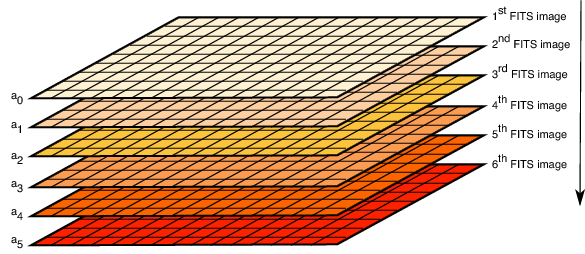
Fig. 6.1 A schematic layout of the fits flat-field cube. This figure is taken from the aXe manual and reproduced here courtesy of Nor Pirzkal.
6.3. Sensitivity Curves
The sensitivity curve provides the conversion between detector units (usually \(\mathrm{e}^-/\mathrm{s}\)) to physical units (usually \(erg/s/cm^2/Å\)), which depends on spectral order by NOT on spatial extent as that is addressed by the flat-field. This can be thought of as a wavelength-dependent zeropoint in flux units. Fig. 6.2 shows the sensitivity curves for several grism and prism modes for several HST instruments.
Note
Although the sensitivity curves have explicit units, they are adjusted by the configurable parameters: fluxscale and fluxunits.
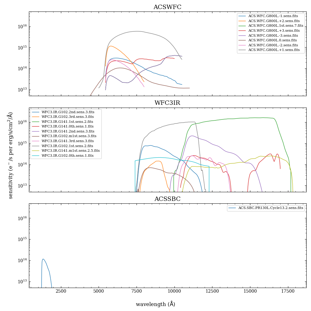
Fig. 6.2 The sensitivity curves for the ACS/WFC, WFC3/IR, and ACS/SBC instruments.