5.1.5. Regions Files for ds9 (Region())

It is occasionally useful to render the two-dimensional WFSS image with spectral traces marked. For this, slitlessutils has the ability to distill the PDT files into a ds9 region file using the module slitlessutils.modules.Region().

To determine the outline of a spectral source in a WFSS image, one should load the images (WFSSCollection()) and sources (SourceCollection()), and then slitlessutils will:

• For every WFSS image:

  • For every detector in the WFSS image:

    • For every source:

      • For every spectral order in question:

        1. load the PDTs for all of the direct imaging pixels associated with the source

        2. decimate over wavelength

        3. make temporary mask with 1 for any pixel present in the decimated PDT

        4. apply a binary closing morphological operator from skimage.ndimage with a square kernel, whose size is set in the slitlessutils.modules.Region() object

        5. find the contours for a highly-connected binary image using scikit-image as a closed polygon

        6. write the polygon into the region file as a ds9 polygon regions

  • Write the region file to disk.

• Output a separate ds9 regions file for each WFSS file and detector combination.

The resulting regions will have their title as the segmentation ID and the spectral order will encoded by the color of the region. Slitlessutils assumes the tab20 colormap from matplotlib, where the bold colors are for positive orders, pastel colors are for negative orders, and the zeroth order will be white (see Fig. 5.8 below). The region filename will be the WFSS image filename with the detector name appended. In Fig. 5.9 we show an example of the first-order traces highlighted.

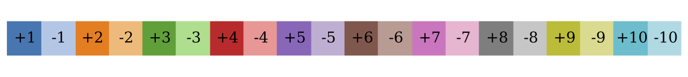
Fig. 5.8 The colors used for spectral orders (indicated as text labels). The bold/pastel colors refer to positive/negative orders, respectively. The zeroth order will be illustrated as white.

Example

import slitlessutils as su

# load the WFSS data
data = su.wfss.WFSSCollection.from_glob('*.fits.gz')

# load the sources
sources = su.sources.SourceCollection(segfile, imgfile)

# instantiate the region module
reg = su.modules.Region(ncpu=1, close_size=12)

# run the module
regfiles = reg(data, sources)

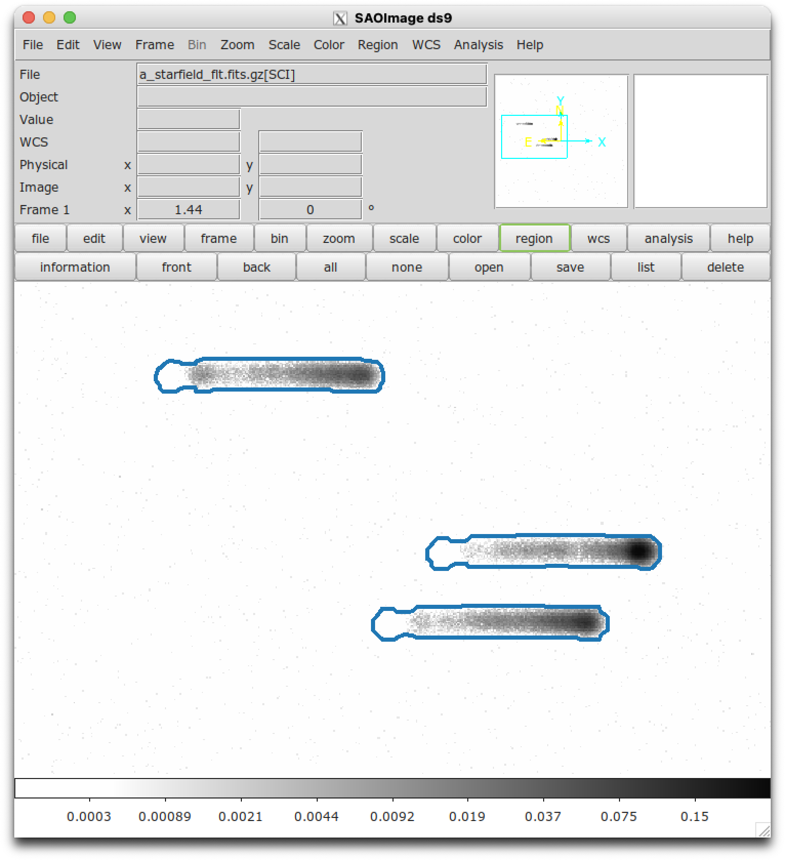
Fig. 5.9 The grayscale image shows the slitlessutils simulation of three Gaussian point sources observed with the ACS/SBC (PR130L). The blue polygons show the regions derived for this scene using slitlessutils.