Background Subtraction

Introduction

The background in a slitless spectroscopic image is generally far more complex than the equivalent for standard imaging, despite likely having the same background SED(s). This occurs because each patch of sky acts as an emitting source and projects its spectrum onto the detector. However, the detector records the sum over all the patches for every spectral order, and since each order has a unique response function, there is a nontrivial shape in the background of a two-dimensional slitless image. This shape is further complicated by the limited distance from the detector that a patch can be and still project light (of any order) onto the detector, which often arises from the finite size of the pick-off mirror (POM) or other optical element (e.g. a baffle). A final confounding issue is that each pixel in the detector likely has a unique, wavelength-dependent flat field, which further modulates the effective brightness from the sky. The net result of these effects is a background map with significant structure (see Fig. 5.2 for an example background for G800L with HST/ACS-WFC).

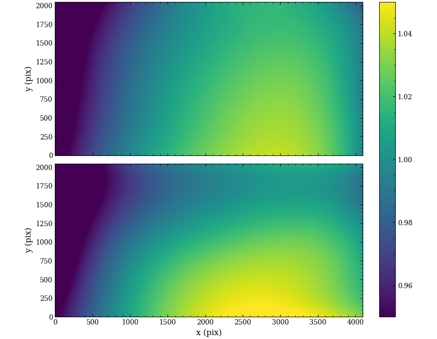
Fig. 5.2 The smoothed global-sky image for the Advanced Camera for Surveys (ACS) G800L grating.

Global-Sky Subtraction

Given the issues inherent in the sky background for wide-field slitless spectroscopy summarized above, the canonical approach to separating this signal from the astrophysical sources of interest is the use of a global-sky image. Here many science and calibration exposures have been combined in a way to remove the sources, and provide a clean image of the sky background. Therefore the present task is to scale this sky image such that it matches the sky pixels in a \({\chi}^2\)-sense. For a single sky image, this multiplicative scaling is given by:

\[\alpha = \frac{\sum_{x,y} w_{x,y}\,S_{x,y}\,B_{x,y}}{\sum_{x,y} w_{x,y}\,B_{x,y}\,B_{x,y}}\]

where \((x,y)\) refer to the WFSS-image pixel positions, \(w_{x,y}\), \(I_{x,y}\), and \(B_{x,y}\) represent the pixel weights (more on this below), wide-field slitless image, and global-sky image, respectively. Therefore sky-subtracted slitless image will be given by

\[B'_{x,y} = \alpha\,B_{x,y}.\]

For a Gaussian likelihood function, the pixel weight are given as the inverse of the uncertainties squared: \(w_{x,y}=U_{x,y}^{-2}\), but are modified for the presence of bad pixels encoded in the data-quality array (DQA) or spectroscopic sources. In the case of a bad-pixel, the weights are set to zero for any pixel with a non-zero value in the DQA. For the sources, the weights are multiplied by an object mask \(\Theta_{x,y}\):

\[\begin{split}\Theta_{x,y} = \left\{ \begin{array}{ll} 0 & \quad \mathrm{if~sky}\\ 1 & \quad \mathrm{if~source} \end{array}\right.\end{split}\]

but is initialized to all sky pixels (ie. \(\Theta_{x,y}=0\)). Now the final weights are:

\[w_{x,y} = \frac{1-\Theta_{x,y}}{U_{x,y}^2}\]

Tip

You may receive the warning:

“The global-sky image (XXXX) is unnormalized YYY. Results will be fine, but the values may be suspect.”

This is a benign warning that background image \(B_{x,y}\) is not normalized to unity, and so \(\alpha\) does not represent a physical quantity but still optimizes the background subtraction. Therefore the subtraction can be trusted, however the \(\alpha\) value has no physical interpretation.

Note

Classical local-sky subtraction (with sky annuli above/below the trace) is generally discouraged, as these regions are often contaminated. Therefore slitlessutils currently has no facility for such operations.

Updating the Object Mask

The presence of the spectra from astrophysical sources complicates the estimation of the scaling parameter, and so they must be masked [1]. In principle, the automatic detection and masking of source spectra could be done in a number of ways, but slitlessutils implements an iterative approach of comparing between a notional scaled background image and the data.

The slitlessutils algorithm for masking objects is:

1. Initialize the background model as a constant value determined from a sigma-clipped median, while masking known bad pixels.

2. Estimate the optimal scaling parameter \(\alpha\) from the above expression.

3. Flag pixels in the object weights by setting pixels in \(\Theta_{x,y}\) with

   \[\left|S_{x,y}-\alpha\,B_{x,y}\right| \geq n_{sig} \,U_{x,y}\]

   where \(n_{sig}\) is a number of sigma for sources.

4. Go to step 2, and repeat until either a maximum number of iterations is reached or the fractional change in \(\alpha\) is below a convergence threshold \(\epsilon\):

   \[\left|\alpha^{(k)} - \alpha^{(k-1)}\right| \leq \epsilon\,\alpha^{(k)}\]

   for iteration \(k\).

A consequence of this iterative approach is the optimized scaling parameter \(\alpha^{(k)}\), which is used to produce the final sky-subtracted WFSS image:

\[S'_{x,y} = S_{x,y} - \alpha^{(k)} B_{x,y}\]

At this point there are two things worth mentioning. Firstly, there are effectively two parameters that govern the global-sky subtraction: \(n_{sig}\) and \(\epsilon\) that control the sigma clipping for sources and convergence tolerance, respectively. Secondly, while the foremost goal was to determine the sky background level, a useful byproduct is the updated object model \(\Theta_{x,y}\), which is saved by default to a file named f"{base}_src.fits".

Example

Here we show a quick example to use the global-sky subtraction for a single grism exposure given by the filename grismfile:

import slitlessutils as su

# perform the global sky subtraction on the filename "grismfile"
su.core.preprocess.background.image(grismfile, inplace=True)

This will update the file in place, as the flag is set: inplace=True, but will additionally write a f"{base}_src.fits" file to disk.

Column-Based Refinement

Coming soon.

Special Notes for WFC3/IR

The above description is for a single-component sky-background spectrum. However, the infrared channel in the Wide-Field Camera 3 (WFC3) instrument on HST is known to exhibit multiple spectral components. Pirzkal & Ryan (2020) derive a separate background image for each spectral component for each infrared grism. These multiple components should be used with the WFC3_Back_Sub utility, as these ideas are not subsumed into slitlessutils. In brief, this requires starting with the RAW files for the grism data, and processing for each visit (WFC3_Back_Sub will group the data by visit).

Important

WFC3/IR data should be sky-subtracted with WFC3_Back_Sub, which requires starting from the RAW files.

Footnotes

[1]

For our present purposes, we do not need to distinguish between the spectral traces of genuine astrophysical objects, cosmic rays, or other deviant pixels — just identify pixels that are not solely sky. However for future analyses (such as spectral extraction), this distinction will become important. See the documentation on cosmic rays for more information.